Frequency Response Analysis
Use the data in tutorial/17_freq_beam.
Analysis Target
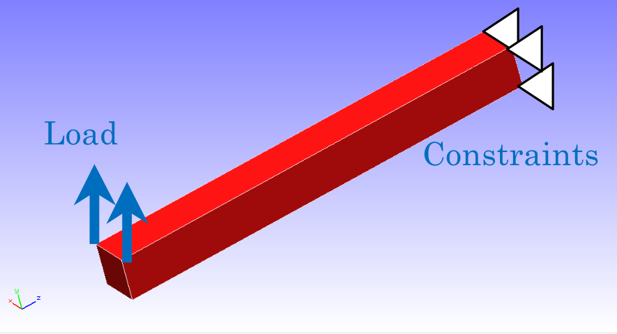
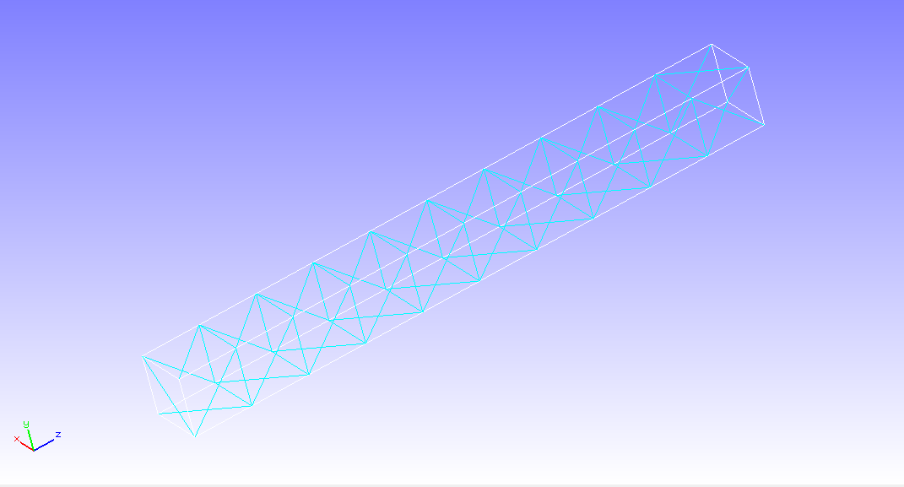
The analysis target is a cantilever beam. Figure 4.17.1 shows the geometry, and Figure 4.17.2 shows the mesh.
| Item | Description | Notes | Reference |
|---|---|---|---|
| Analysis type | Frequency response analysis | !SOLUTION,TYPE=EIGEN !SOLUTION,TYPE=DYNAMIC | |
| Number of nodes | 55 | ||
| Number of elements | 126 | ||
| Element type | 4-node linear tetrahedral element | !ELEMENT,TYPE=341 | |
| Material name | Material-1 | !MATERIAL,NAME=Material-1 | |
| Boundary conditions | Restraint, concentrated load, eigenmodes | !EIGENREAD | |
| Matrix solver | CG/SSOR | !SOLVER,METHOD=CG,PRECOND=1 |
Analysis Setup
Fully constrain one end of the cantilever beam and apply concentrated loads to two nodes at the opposite end to perform a frequency response analysis.
First perform modal analysis through the tenth mode under the same boundary conditions. Then perform the frequency response analysis using the eigenvalues and eigenvectors through the fifth mode. The Analysis Control Data for the frequency response analysis are shown below.
Analysis Control Data beam_eigen.cnt
#  Control File for FISTR
!VERSION
 3
!WRITE,RESULT
!WRITE,VISUAL
!SOLUTION, TYPE=EIGEN
!EIGEN
 10, 1.0E-8, 60
!BOUNDARY
_PickedSet4, 1, 3, 0.0
!SOLVER,METHOD=CG,PRECOND=1,ITERLOG=NO,TIMELOG=YES
 10000, 1
 1.0e-8, 1.0, 0.0
!VISUAL,method=PSR
!surface_num=1
!surface 1
!output_type=VTK
!END
Analysis Control Data beam_freq.cnt
#  Control File for FISTR
!VERSION
 3
!WRITE,RESULT
!WRITE,VISUAL
!SOLUTION, TYPE=DYNAMIC
!DYNAMIC
 11 , 2
 14000, 16000, 20, 15000.0
 0.0, 6.6e-5
 1, 1, 0.0, 7.2E-7
 10, 2, 1
 1, 1, 1, 1, 1, 1
!EIGENREAD
 eigen_0.log
 1, 5
!BOUNDARY
_PickedSet4, 1, 3, 0.0
!FLOAD, LOAD CASE=2
_PickedSet5, 2, 1.
!FLOAD, LOAD CASE=2
_PickedSet6, 2, 1.
!SOLVER,METHOD=CG,PRECOND=1,ITERLOG=NO,TIMELOG=YES
 10000, 1
 1.0e-8, 1.0, 0.0
!VISUAL,method=PSR
!surface_num=1
!surface 1
!output_type=VTK
!END
Analysis Procedure
First, rename the modal-analysis Overall Control Data file hecmw_ctrl_eigen.dat to hecmw_ctrl.dat, then run the modal analysis.
Next, rename the frequency-response Overall Control Data file hecmw_ctrl_freq.dat to hecmw_ctrl.dat and the modal-analysis result log file 0.log to eigen_0.log (as specified in the Analysis Control Data for the frequency response analysis), then run the frequency response analysis.
cp hecmw_ctrl_eigen.dat hecmw_ctrl.dat
fistr1 -t 4
mv 0.log eigen_0.log
cp hecmw_ctrl_freq.dat hecmw_ctrl.dat
fistr1 -t 4
Analysis Results
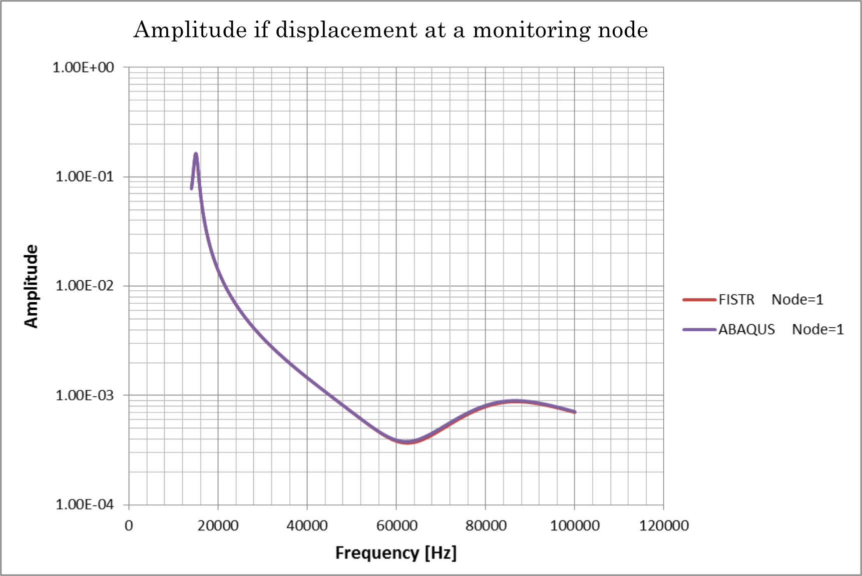
Figure 4.17.3 shows the relationship between frequency and displacement amplitude at the monitoring node (node 1) specified in the Analysis Control Data, plotted using Microsoft Excel. An excerpt from the analysis result log file is shown below as numerical output.
Analysis Result Log 0.log (Frequency Response Analysis)
 fstr_setup: OK
 Rayleigh alpha:   0.0000000000000000
 Rayleigh beta:   7.1999999999999999E-007
 read from=eigen_0.log
 start mode=           1
 end mode=           5
 start frequency:   14000.000000000000
 end frequency:   16000.000000000000
 number of the sampling points          20
 monitor nodeid=           1
   14100.000000000000      [Hz] :    8.3935554529723885E-002
   14100.000000000000      [Hz] :            1 .res
   14200.000000000000      [Hz] :    9.1211083509607632E-002
   14200.000000000000      [Hz] :            2 .res
   14300.000000000000      [Hz] :    9.9579777896922961E-002
   14300.000000000000      [Hz] :            3 .res
   14400.000000000000      [Hz] :   0.10914967594967491
   14400.000000000000      [Hz] :            4 .res
   14500.000000000000      [Hz] :   0.11992223203326918
   14500.000000000000      [Hz] :            5 .res
   14600.000000000000      [Hz] :   0.13164981801806747
   14600.000000000000      [Hz] :            6 .res
   14700.000000000000      [Hz] :   0.14360931008440975
   14700.000000000000      [Hz] :            7 .res
   14800.000000000000      [Hz] :   0.15436500205940235
   14800.000000000000      [Hz] :            8 .res
   14900.000000000000      [Hz] :   0.16180768408076251
   14900.000000000000      [Hz] :            9 .res
   15000.000000000000      [Hz] :   0.16388019610373711
   15000.000000000000      [Hz] :           10 .res
   15100.000000000000      [Hz] :   0.15982110598747551
   15100.000000000000      [Hz] :           11 .res
   15200.000000000000      [Hz] :   0.15074650286398145
   15200.000000000000      [Hz] :           12 .res
   15300.000000000000      [Hz] :   0.13885370598993371
   15300.000000000000      [Hz] :           13 .res
   15400.000000000000      [Hz] :   0.12618976409021948
   15400.000000000000      [Hz] :           14 .res
   15500.000000000000      [Hz] :   0.11405716994112736
   15500.000000000000      [Hz] :           15 .res
   15600.000000000000      [Hz] :   0.10306231010139058
   15600.000000000000      [Hz] :           16 .res
   15700.000000000000      [Hz] :    9.3374567545990342E-002
   15700.000000000000      [Hz] :           17 .res
   15800.000000000000      [Hz] :    8.4945897112663621E-002
   15800.000000000000      [Hz] :           18 .res
   15900.000000000000      [Hz] :    7.7641947016103510E-002
   15900.000000000000      [Hz] :           19 .res
   16000.000000000000      [Hz] :    7.1307642422355627E-002
   16000.000000000000      [Hz] :           20 .res
 start time:   0.0000000000000000
 end time:   6.6000000000000005E-005
 frequency:   15000.000000000000
 node id:           1
 num disp:          10
 time=   0.0000000000000000       :            1 .res
 time=   0.0000000000000000       :            1 .vis
 time=   6.6000000000000003E-006  :            2 .res
 time=   6.6000000000000003E-006  :            2 .vis
 time=   1.3200000000000001E-005  :            3 .res
 time=   1.3200000000000001E-005  :            3 .vis
 time=   1.9800000000000000E-005  :            4 .res
 time=   1.9800000000000000E-005  :            4 .vis
 time=   2.6400000000000001E-005  :            5 .res
 time=   2.6400000000000001E-005  :            5 .vis
 time=   3.3000000000000003E-005  :            6 .res
 time=   3.3000000000000003E-005  :            6 .vis
 time=   3.9600000000000000E-005  :            7 .res
 time=   3.9600000000000000E-005  :            7 .vis
 time=   4.6200000000000005E-005  :            8 .res
 time=   4.6200000000000005E-005  :            8 .vis
 time=   5.2800000000000003E-005  :            9 .res
 time=   5.2800000000000003E-005  :            9 .vis
 time=   5.9400000000000000E-005  :           10 .res
 time=   5.9400000000000000E-005  :           10 .vis