Modal Analysis
Generalized Eigenvalue Problem
For free-vibration analysis of a continuum, the structure is spatially discretized and modeled as a multi-degree-of-freedom system with lumped masses, as shown in Figure 2.3.1. For an undamped free-vibration problem, the governing equation (equation of motion) is as follows.
Here, \(u\) is the generalized displacement vector, \(M\) is the mass matrix, and \(K\) is the stiffness matrix. Let \(\omega\) be the natural angular frequency, let \(a\) and \(b\) be arbitrary constants that are not both zero, and let \(x\) be a vector. Define the function
Its second derivative is
Substituting Equation \(\eqref{eq:2.3.2}\) and Equation \(\eqref{eq:2.3.3}\) into Equation \(\eqref{eq:2.3.1}\) gives
This gives the equation above.
For a nontrivial vibration, \(a \sin \omega t + b \cos \omega t\) is not identically zero.
Therefore, the relation above follows. Thus, setting \(\lambda=\omega^2\) gives
This gives the equation above.
The scalar \(\lambda\) is called an eigenvalue, the vector \(x\) is called an eigenvector, and the problem expressed by Equation \(\eqref{eq:2.3.5}\) is called a generalized eigenvalue problem.
The natural angular frequency \(\omega\) is obtained from the eigenvalue \(\lambda=\omega^2\), and the corresponding eigenvector \(x\) represents a mode shape.

Figure 2.3.1 Example of a Multi-Degree-of-Freedom System for Undamped Free Vibration
Matrix Properties and Assumptions
For the generalized eigenvalue problem \(Kx=\lambda Mx\) obtained in the preceding section, this manual assumes that the matrices are symmetric. For complex matrices, this corresponds to Hermitian matrices; for real matrices, it corresponds to symmetric matrices.
Let \(k_{ij}\) be the \(ij\) entry of matrix \(K\). The Hermitian property is
expressed by the equation above, where \(\bar{k}_{ji}\) is the complex conjugate of \(k_{ji}\). For real matrices, this relation becomes \(k_{ij}=k_{ji}\).
A real symmetric matrix \(H\) is positive definite if, for every nonzero vector \(x\),
the inequality above holds. In this case, all eigenvalues of \(H\) are positive.
In a structural eigenvalue problem, the mass matrix \(M\) is normally treated as positive definite. The stiffness matrix \(K\), however, may be positive semidefinite depending on the constraints and may have zero eigenvalues corresponding to rigid-body modes.
Shifted Inverse Iteration
In practical finite element structural analysis, all eigenvalues are generally unnecessary; at most a few low-order eigenvalues are often sufficient. HEC-MW is intended for large-scale problems, for which the matrices are large and extremely sparse, with many zero entries. It is therefore important to compute the eigenvalues of low-order modes efficiently with these characteristics in mind.
For a shift \(\sigma\), if \(-\sigma\) is not an eigenvalue and \(K+\sigma M\) is nonsingular, Equation \(\eqref{eq:2.3.5}\) can be transformed as follows.
This transformation leaves the eigenvector \(x\) unchanged and maps the eigenvalue \(\lambda\) to \(1/(\lambda+\sigma)\).
Consequently, the closer \(\lambda\) is to \(-\sigma\), the larger the absolute value of the transformed eigenvalue. For a structural eigenvalue problem, \(\lambda \geq 0\) and \(\sigma \geq 0\), so the lowest eigenvalue is mapped to the eigenvalue with the largest absolute value. Using this property, applying to Equation \(\eqref{eq:2.3.8}\) an iterative method that tends to converge first to eigenvalues of large absolute value allows the low-order eigenvalues to be obtained efficiently in ascending order.
This method is called shifted inverse iteration.
For analyses with constraints, FrontISTR sets \(\sigma = 0\), and Equation \(\eqref{eq:2.3.8}\) becomes \(K^{-1} M x = \frac{1}{\lambda} x\), that is, unshifted inverse iteration. In unconstrained free-free analysis, \(K\) is singular because it has zero eigenvalues corresponding to rigid-body modes; assigning a positive value to \(\sigma\) regularizes \(K+\sigma M\). The value of \(\sigma\) is specified by SIGMA in !EIGEN.
Lanczos Method
Rationale (Comparison with the Jacobi Method)
The Jacobi method is a well-known classical method.
It is effective when the matrix is small and dense. However, because the matrices handled by HEC-MW are large and sparse, the Jacobi method is not adopted; instead, the Lanczos iterative method is used.
Algorithm and Features
Proposed by C. Lanczos in the 1950s, this method is an algorithm for tridiagonalizing a matrix and has the following features.
- It is an iterative method and can perform the computation while keeping the matrix sparse.
- Its operations consist primarily of matrix-vector products, making it well suited to parallelization.
- It is well suited to geometric domain decomposition associated with finite element meshes.
- It can perform efficient computations by limiting the number of eigenvalues or the range of modes to be obtained.
The Lanczos method starts from an initial vector, successively constructs orthogonal vectors, and obtains a basis for a Krylov subspace.
In finite-precision arithmetic, roundoff error can cause the vectors to lose orthogonality. To suppress this effect, the FrontISTR implementation reorthogonalizes each vector against the Lanczos basis vectors already obtained.
Geometric Interpretation (Krylov Subspace)
Applying the following variable transformations to Equation \(\eqref{eq:2.3.8}\),
the problem can be rewritten as
This gives the equation above.
For an arbitrary nonzero vector \(q_0\),
the space spanned by these vectors,
is called a Krylov subspace.
The Lanczos method constructs a basis for this Krylov subspace successively.
FrontISTR uses the following inner product associated with the mass matrix \(M\)
to orthonormalize the basis. The inner product \(\langle x,y\rangle\) and norm \(\|x\|\) shown in the following figures are interpreted in FrontISTR calculations as this \(M\)-inner product and the corresponding \(M\)-norm
respectively.
Apply the linear transformation defined by matrix \(A\) to an arbitrary vector \(q_0\), as shown in Figure 2.3.2.
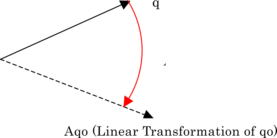
Figure 2.3.2 Linear Transformation of \(q_0\) by Matrix \(A\)
The transformed vector is orthogonalized within the space spanned by it and the original vector. Specifically, Gram-Schmidt orthogonalization is performed as shown in Figure 2.3.3. Let the resulting vector be \(r_1\); normalizing it gives \(q_1\).
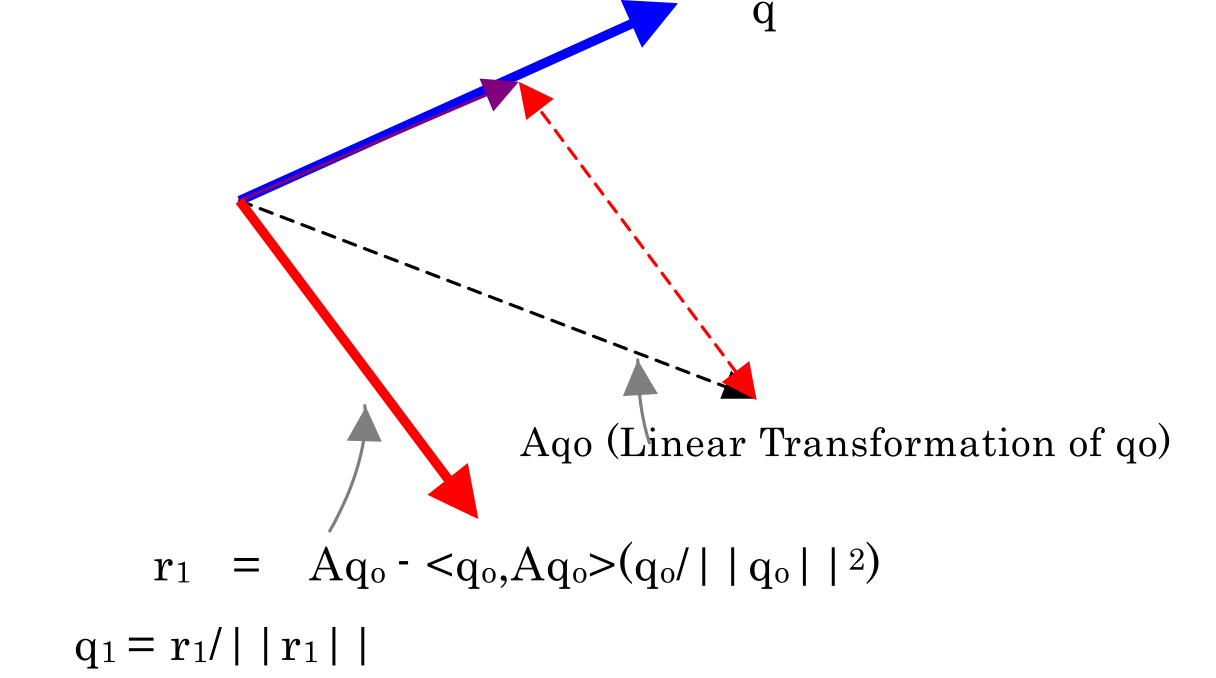
Figure 2.3.3 Vector \(q_1\) Orthogonal to \(q_0\)
The same procedure obtains \(q_2\) from \(q_1\). Here, \(q_2\) is orthogonal to both \(q_1\) and \(q_0\), as shown in Figure 2.3.4.
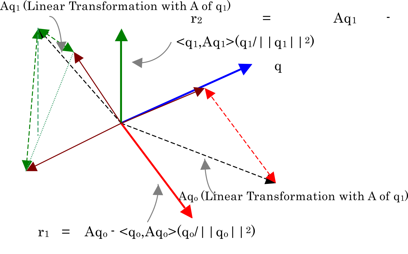
Figure 2.3.4 Vector \(q_2\) Orthogonal to \(q_1\) and \(q_0\)
In this way, the Lanczos method successively constructs an orthonormal basis for the Krylov subspace. In theory, the symmetry of the eigenvalue problem allows this iteration to be expressed as a three-term recurrence involving the most recent basis vectors.
The FrontISTR implementation, however, reorthogonalizes each vector against the Lanczos basis vectors already obtained using the \(M\)-inner product to suppress loss of orthogonality caused by finite-precision arithmetic.
Tridiagonalization
In FrontISTR's Lanczos iteration, the basis vectors are orthonormalized with respect to the \(M\)-inner product described in the preceding section, so
the relation above holds.
Using matrix \(A\) from Equation \(\eqref{eq:2.3.10}\), the theoretical Lanczos iteration is
represented by the three-term recurrence above.
First, \(\alpha_i\) is defined as follows.
Next, define the provisional residual as
shown above.
To suppress loss of orthogonality caused by finite-precision arithmetic, the FrontISTR implementation reorthogonalizes \(\tilde{r}_{i+1}\) against the Lanczos basis vectors already obtained using the \(M\)-inner product. If \(r_{i+1}\) is the residual after reorthogonalization, then
the relations above hold.
Collect the \(m\) basis vectors obtained by the Lanczos iteration into
Then, after a finite number of Lanczos iterations,
the relation above holds.
Here, \(e_m\) is the \(m\)-dimensional unit vector whose \(m\)-th component is 1 and whose other components are zero, and
is a symmetric tridiagonal matrix.
Thus, the eigenvalues of the original large-scale eigenvalue problem can be approximated by computing the eigenvalues of the tridiagonal matrix \(T_m\).
See Also
- Frequency Response Analysis — Frequency response using modal-analysis results
- Analysis Types — Functional overview of modal analysis