Elastic Static Analysis Examples Using Realistic Models
Analysis Models
Table 9.2.1 lists the verification examples using realistic models for elastic static analysis. The model geometries, with some exceptions, are also shown in Figures 9.2.1 through 9.2.5. A separate direct solver is required to run the examples using element types 731 and 741.
Table 9.2.1 Verification examples using realistic models for elastic static analysis
| Case Name | Element Type | Verification Model | Number of Nodes | Degrees of Freedom |
|---|---|---|---|---|
| EX01A | 342 | Connecting rod (100,000 nodes) | 94,074 | 282,222 |
| EX01B | 342 | Connecting rod (330,000 nodes) | 331,142 | 993,426 |
| EX02 | 361 | Block with a hole | 37,386 | 112,158 |
| EX03 | 342 | Turbine blade | 10,095 | 30,285 |
| EX04 | 741 | Cylindrical shell | 10,100 | 60,600 |
| EX05A | 731 | Wine glass (coarse) | 7,240 | 43,440 |
| EX05B | 731 | Wine glass (medium) | 48,803 | 292,818 |
| EX05C | 731 | Wine glass (fine) | 100,602 | 603,612 |
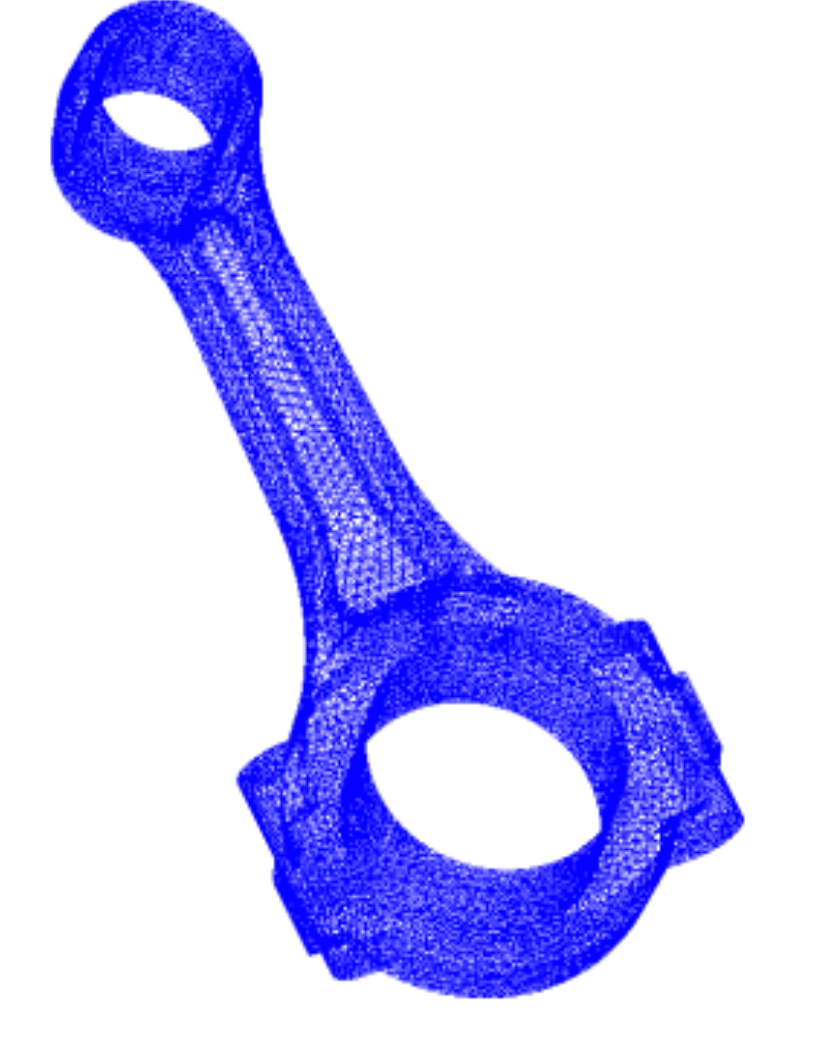
Figure 9.2.1 Connecting rod (EX01A)
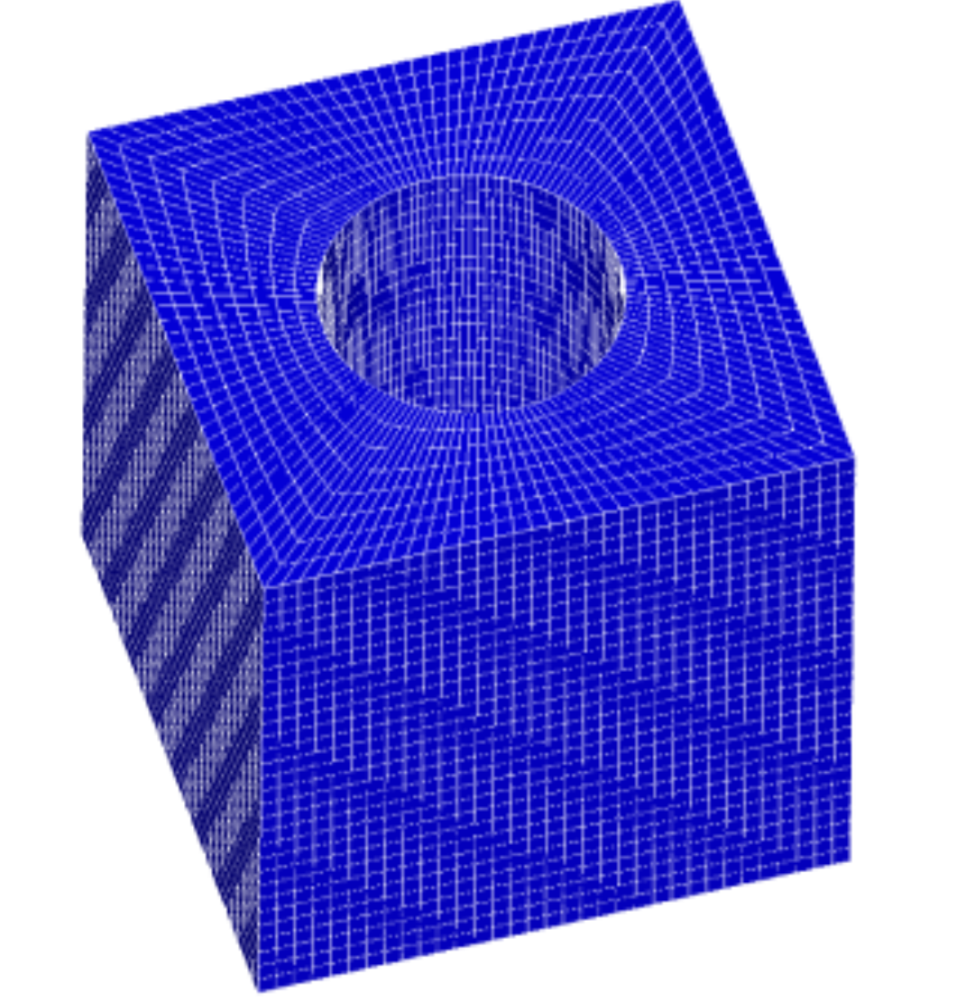
Figure 9.2.2 Block with a hole (EX02)
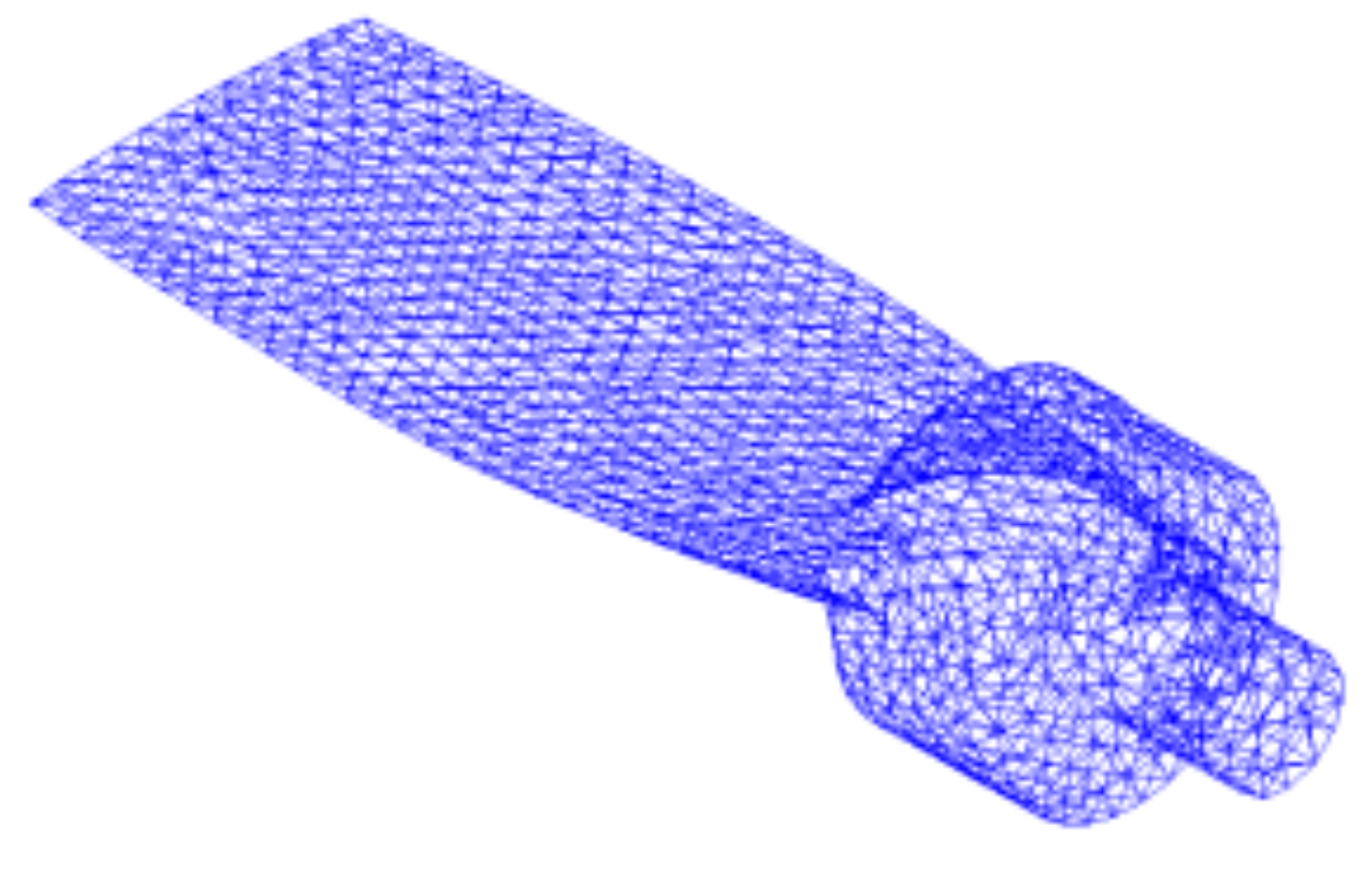
Figure 9.2.3 Turbine blade (EX03, EX06)
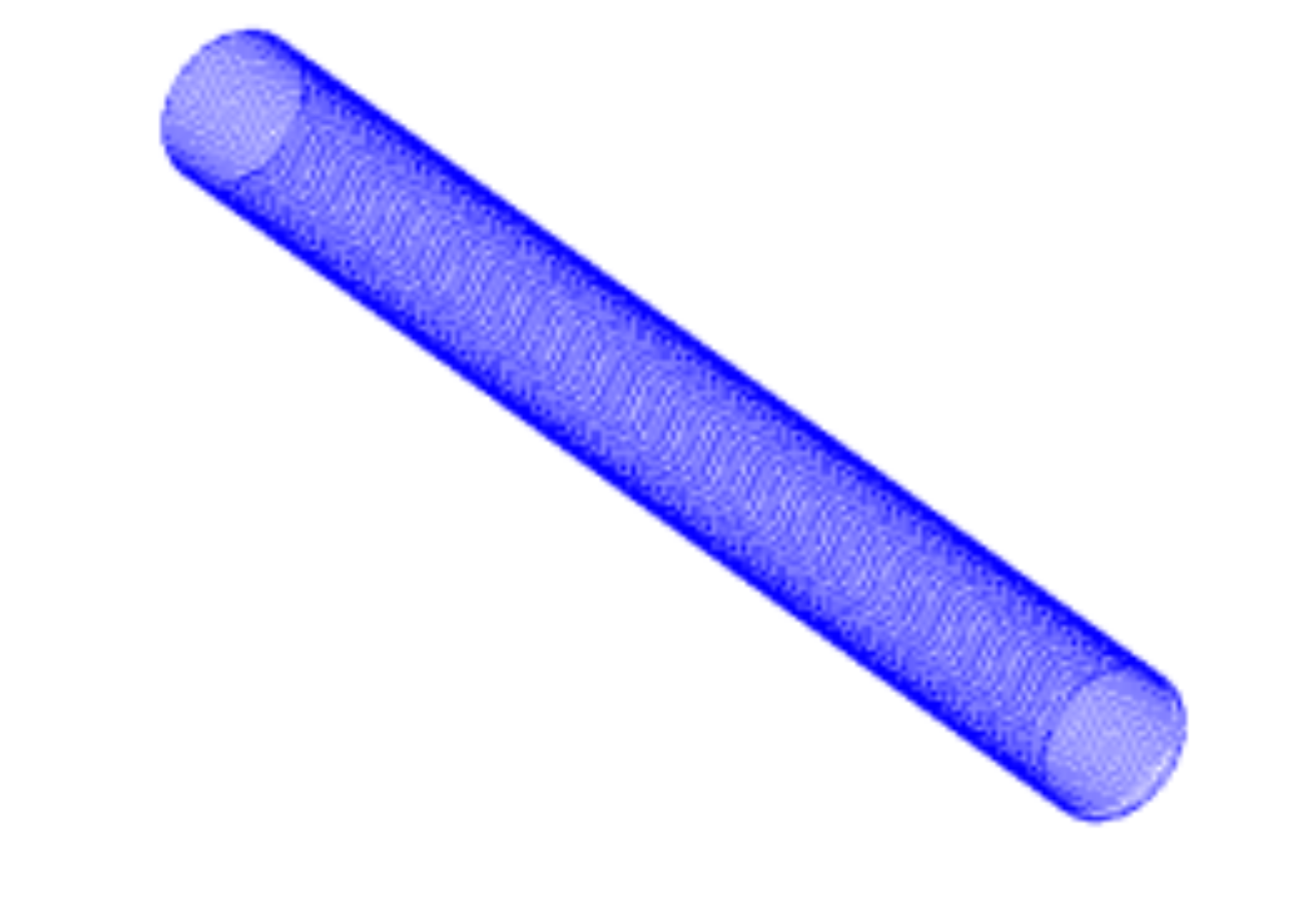
Figure 9.2.4 Cylindrical shell (EX04, EX09)
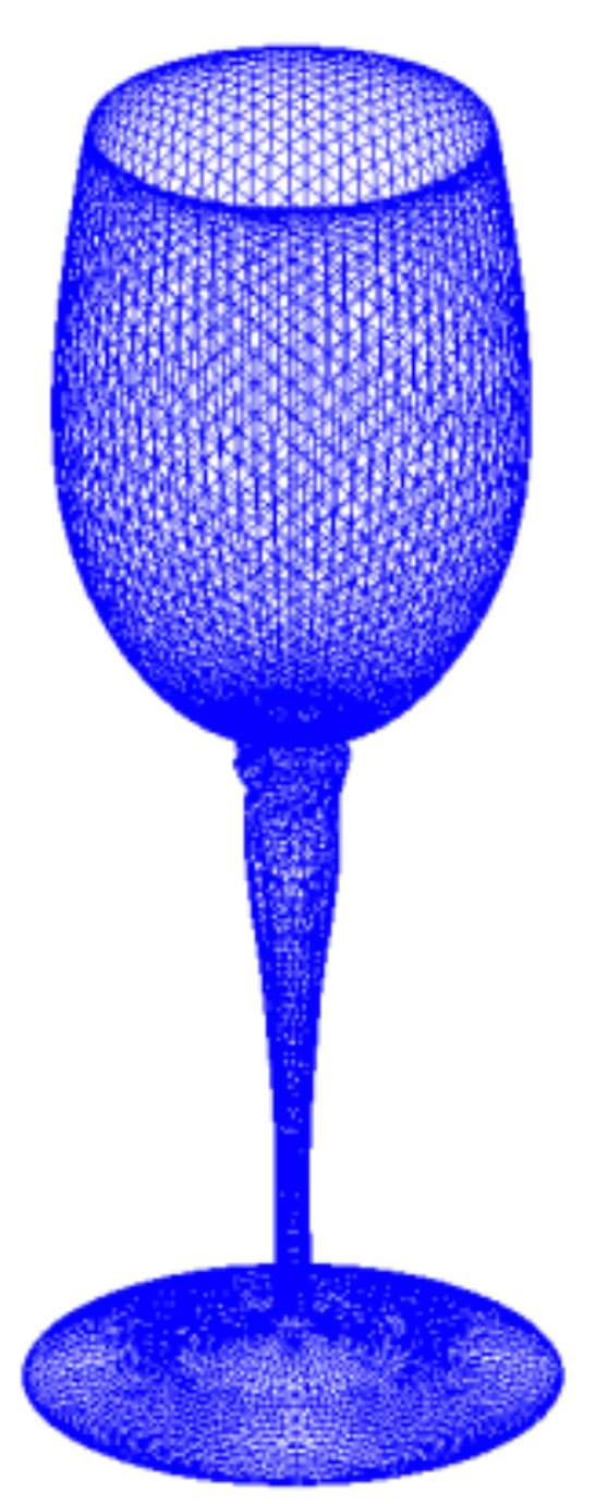
Figure 9.2.5 Wine glass (EX05, EX10A)
Analysis Results
Example Analysis Results
Examples of the analysis results are shown in Figures 9.2.6 through 9.2.9.
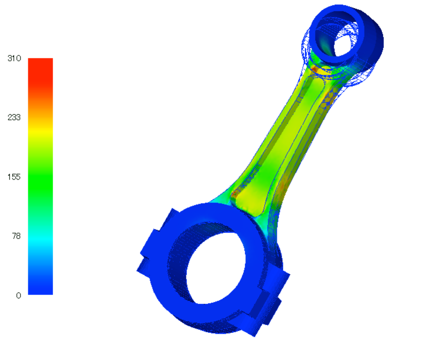
Figure 9.2.6 EX01A analysis results (Mises stress and deformed shape; deformation scale factor: 10)
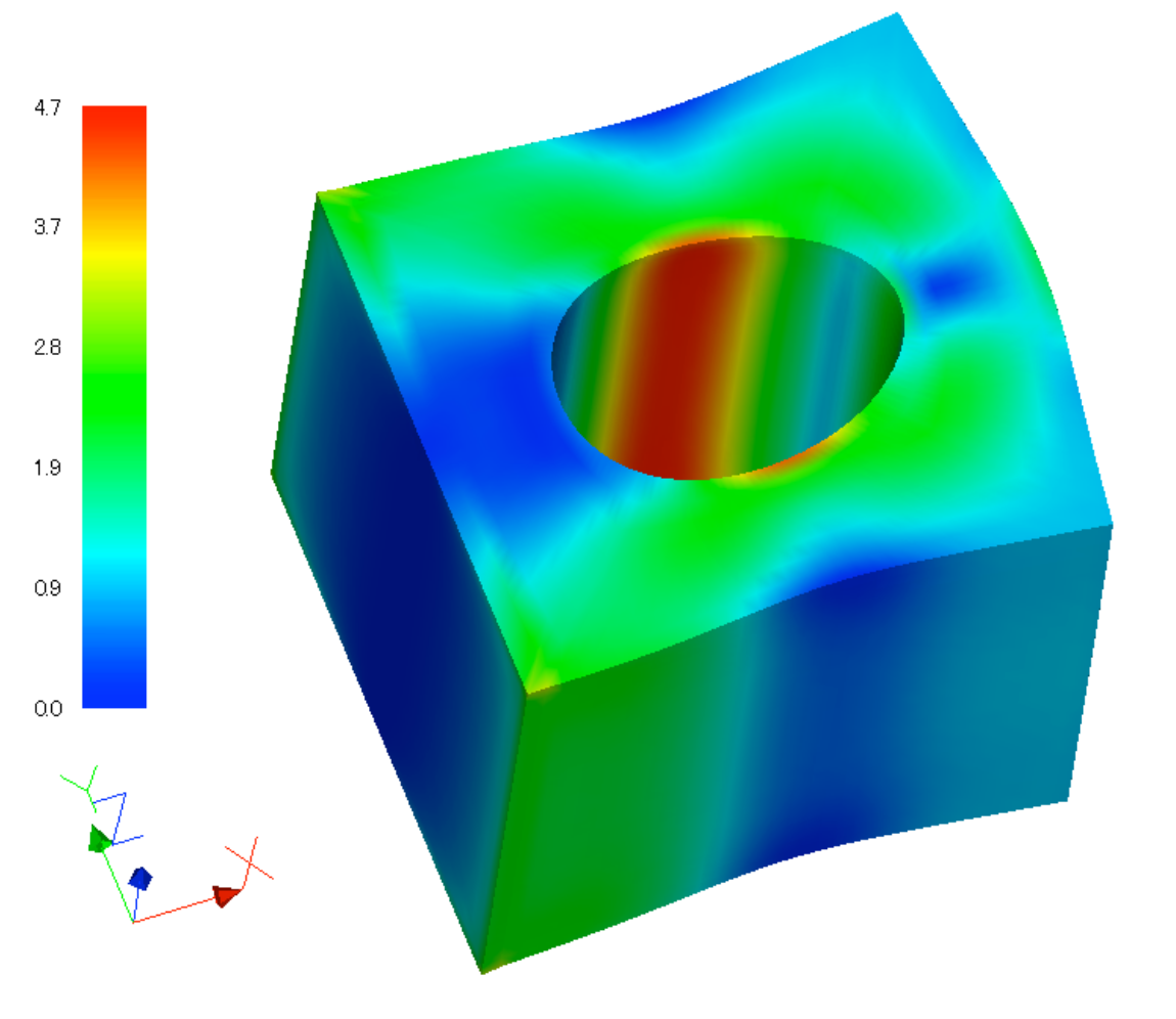
Figure 9.2.7 EX02 analysis results (Mises stress and deformed shape; deformation scale factor: 100)
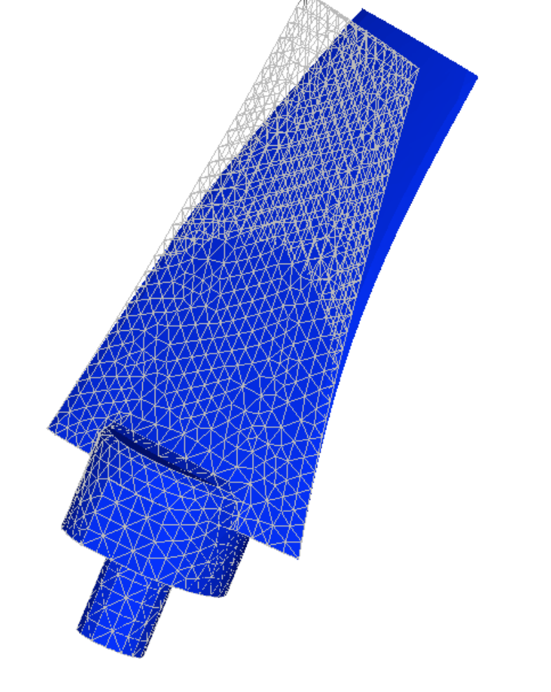
Figure 9.2.8 EX03 analysis results (deformed shape; deformation scale factor: 10)
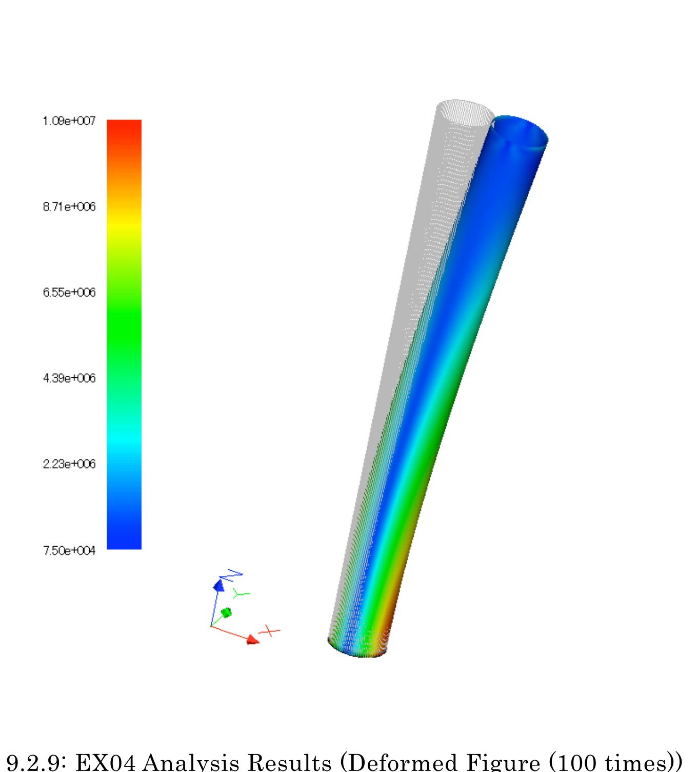
Figure 9.2.9 EX04 analysis results (deformed shape; deformation scale factor: 100)
Analysis Performance Verification Results Using Example EX02
A model equivalent to the EX02 block-with-a-hole verification model was analyzed using general-purpose commercial software. Figure 9.2.10 compares the maximum and minimum stress-component values with those obtained by FrontISTR. The figure shows that the stress components agree very closely.
Next, the effect of domain decomposition on the stress distribution was investigated. The RCB method was used to divide the model into two parts along each of the X, Y, and Z axes, for a total of eight domains. Figure 9.2.11 shows the decomposition. Figure 9.2.12 shows the stress distributions obtained using a single domain and an eight-domain decomposition.
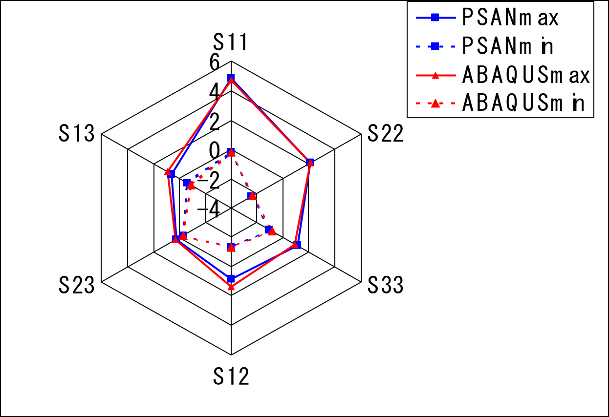
Figure 9.2.10 Comparison of EX02 stress components with general-purpose commercial software
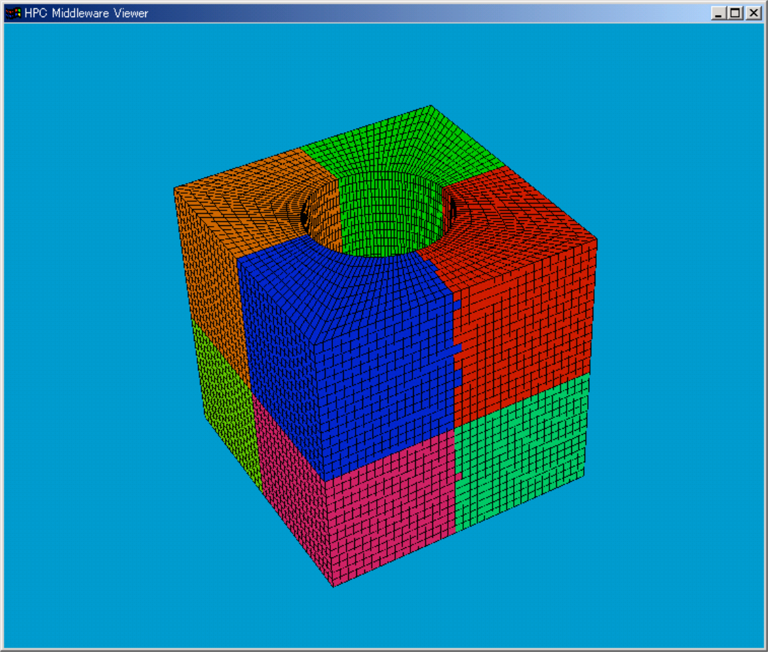
Figure 9.2.11 EX02 divided into eight domains using the RCB method
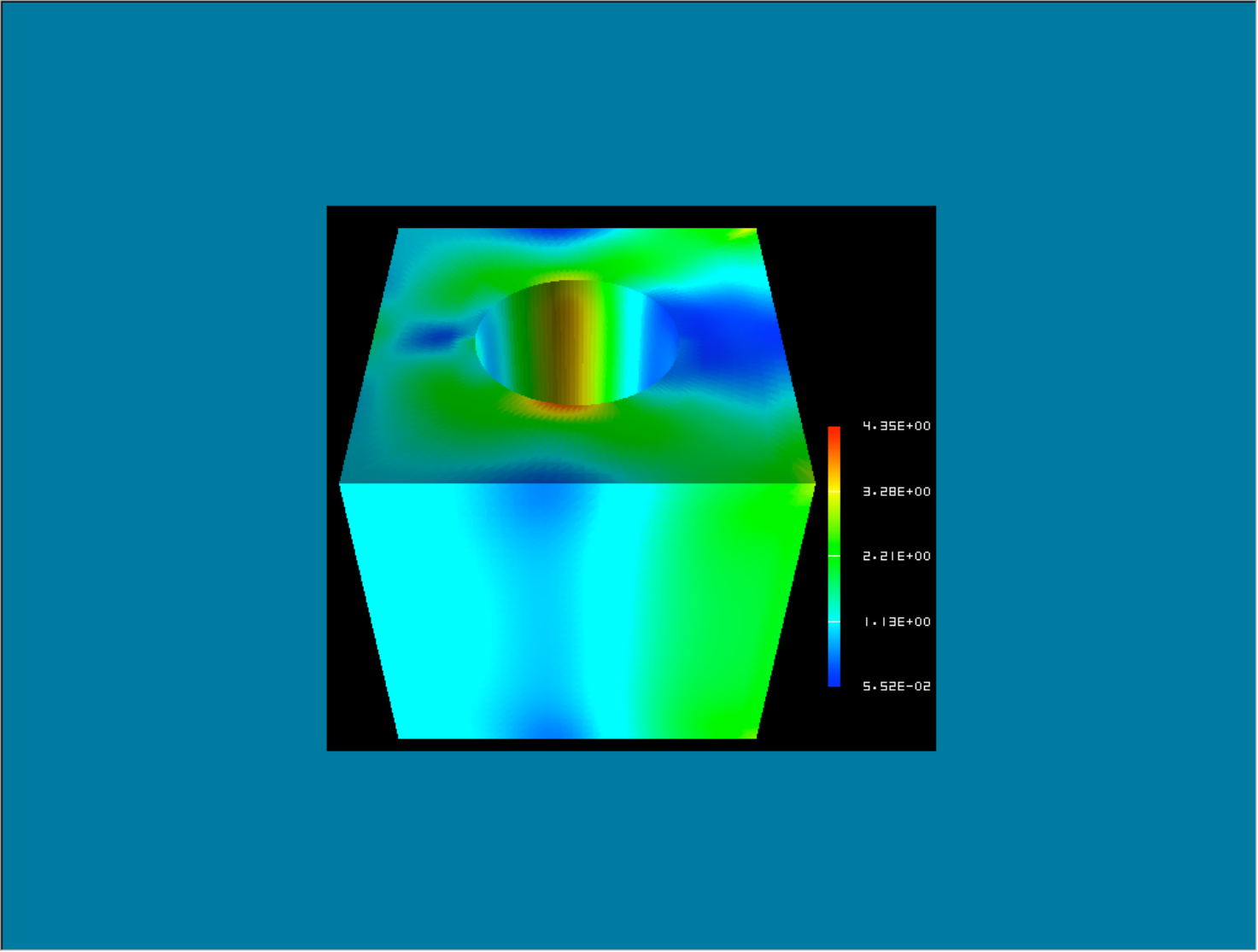
Figure 9.2.12 Difference in Mises stress distribution due to domain decomposition
Figure 9.2.12 shows no difference between the two results; they agree completely.
Table 9.2.2 compares execution times for the HEC-MW solver settings used. Figure 9.2.13 also shows the convergence history until the solution is obtained.
Table 9.2.2 Comparison of execution times using HEC-MW solvers
| Solver | Execution Time (s) |
|---|---|
| CGI | 38.79 |
| CGscale | 52.75 |
| BCGS | 60.79 |
| CG8 | 6.65 |
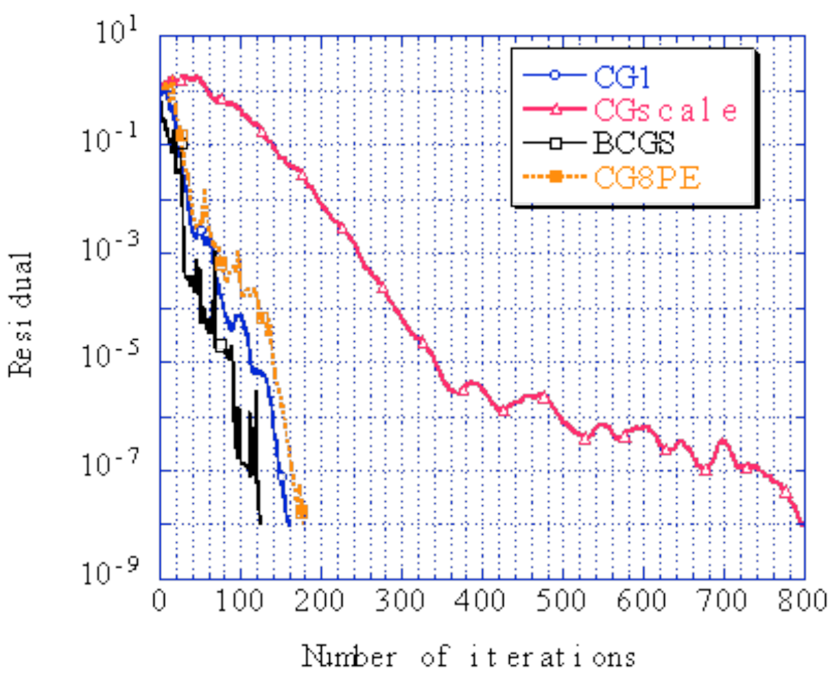
Figure 9.2.13 Comparison of convergence histories using HEC-MW solvers (convergence threshold: \(1.0 \times 10^{-8}\))
Computation Time Comparison Using Verification Example EX01A
Verification example EX01A (connecting rod) was used to evaluate the speedup in computation achieved by domain decomposition. The computation used a 24-node cluster computer with Xeon 2.8 GHz processors. The results are shown in Figure 9.2.14. The figure shows that computation speed increases in proportion to the number of domains.
Differences in computation time between computer environments were also investigated. The results are shown in Table 9.2.3.

Figure 9.2.14 Speedup from domain decomposition
Table 9.2.3 Comparison of computation times by computer (1 CPU)
| CPU | Frequency (GHz) | OS | CPU Time (s) | solver time (s) |
|---|---|---|---|---|
| Xeon | 2.8 | Linux | 850 | 817 |
| Pentium III | 0.866 | Win2000 | 2008 | 1980 |
| Pentium M | 0.760 | WinXP | 1096 | 1070 |
| Pentium 4 | 2.0 | WinXP | 802 | 785 |
| Pentium 4 | 2.8 | WinXP | 738 | 718 |
| Celeron | 0.700 | Win2000 | 2252 | 2215 |
| Pentium 4 | 2.4 | WinXP | 830 | 804 |